resources & deployment

intro

  • Big 3 categories of software:
    1. Analysis code — running Python code once on some data to get results
    2. Application — continuously running the code, like a website
    3. Systems — how to manage resources such as storage space
  • Systems resources:
    • compute -> CPU, GPU
      • CPUs can each have multiple cores, which can be independently executing “core code” (machine code)
      • More cores means that more tasks can be run simultaneously
      • High level code -> compiled to bytecode -> ran by a VM -> VM is running on a core
      • GPU has many cores that are coordinated and slow because they have to run together
      • Cost measurement: FLOPS (floating-point operations per second)
    • mem -> RAM
      • RAM stores bits
      • Small, volatile (lost upon reboot) and fast
    • storage -> HDD, SSD
      • Data read/written in blocks of many bytes/blocks
      • Large, nonvolatile, slow
      • How fast can be read/write data? This is measured in throughput
    • network -> NIC (network interface card)
      • Data access speed can be based on network topology — which servers are physically closest
  • How do we efficiently utilize the four above resources?
    1. Scale UP: get more mem/compute power
    2. Scale OUT: cluster machines (expensive)

deployment

(linux)

  • which where something is installed / located
  • shebang line tells you what interpreter should run the code
  • | pipe character chains output from one program to the input of another program
    • programs don’t wait for the previous one to conclude, they use streams
  • > redirects input/output &> out.txt sends stdout and stderr to out.txt 2> just sends stderr somewhere
  • & sends program to the background to run asynchronously
  • wc word count produces lines words chars
  • grep search
  • find finds all files wrt current dir
  • >> append to a file instead of overwriting it with >
  • ps lists running processes
  • kill [id] kills a process by id
  • pkill [name] kills a process by name
  • htop memory usage
  • df -h storage usage
  • lsof list open files, shows every file that every program has open
    • -i tcp shows which programs are running using tcp

(docker)

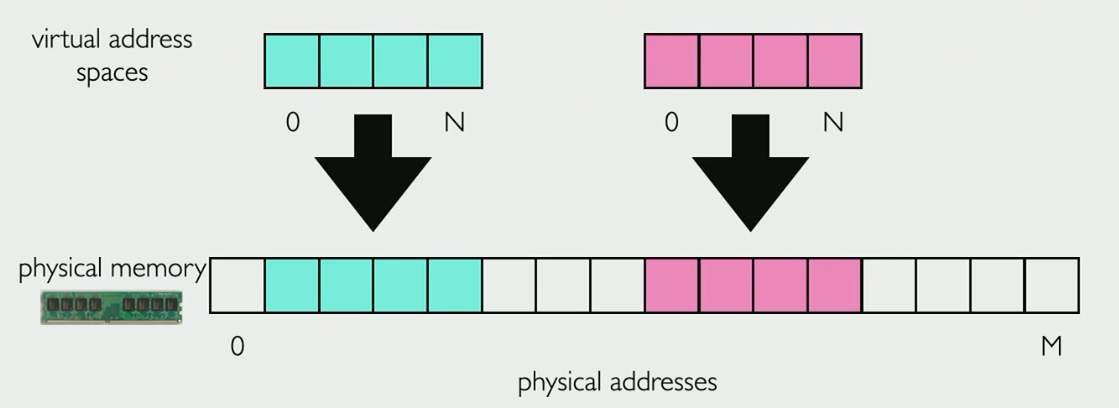
  • Virtualization is the idea that processes are given private resources such as memory or hardware
    • One example is virtual address spaces which are chunks of memory in a larger block of memory, another example is a VM
  • Docker is a way of creating lightweight virtual operating systems, which are called containers
  • The purpose of containers / VMs are to create sandboxes which can run code in an isolated environment
    • For example, running malicious code in a sandbox will not affect anything outside of the sandbox
  • Docker image: a snapshot of a container
    • Containers can be created on your VM from an image
    • Dockerfiles set up environments
      • Dockerfiles will cache intermediate progress, so it’s good practice to put stuff that’s stable at the top, and stuff that’s constantly changing near the bottom of the Dockerfile
  • Use docker run -it IMAGE_NAME bash to get an interactive terminal to run inside a docker container
  • Use docker run IMAGE_NAME sh -c "COMMAND" to run a command inside an image without going into the image
  • Useful troubleshooting commands: logs, exec, stats, kill
  • Each container has its own set of ports
    • If we have two containers, lo and ens0, then there is a port 80 for each of them
    • We can manually map ports from the laptop to a virtual machine, which would allow the user to specify which port 80 they want to use
  • Docker orchestration is for deploying many containers (cluster) that are cooperating, ie: Kubernetes or ßDocker compose
    • Create a file named docker-compose.yml to get started
example docker compose file
services:
    jupyter:
        image: myimg
        deploy:
            replicas: 3
    # TODO: other processes

memory resources

(caching)

  • There is latency when loading data from RAM into CPU, the solution to this is the cache “hot” data
  • Caching is a resource tradeoff — if I cache a file, I avoid rereading from storage, but I’m using up memory
  • What do we cache? Data/webpages that we need to access repeatedly
  • When do we cache? The first time we read something, it is added to the cache
  • When do we remove (evict) from the cache? Depends, there are several policies
    • Why do we evict? Limited cache space
    • Random: remove cache entry at random
    • FIFO (first in, first out): remove whatever has been in the cache the longest
    • LRU (least recently used): remove the cache item that was accessed the longest ago
  • FIFO and LRU are bad when you need to keep scanning the same data repeatedly because you can have a situation where you evict the values that you need next
    • Cache size = 4, Data = [1,2,3,4,5,1,2,3,4,5], then the hit rate is 0%
  • Avg latency = (hit% * hit latency) + (miss% + miss latency)

compute resources

(pytorch numbers)

  • Specify exactly how many bits are used for the numbers we’re working with (uint8, float32, etc)
    • Tradeoffs: precision, range, memory
  • Numbers in PyTorch are called “tensors”
  • Ints will overflow/underflow, floats will return as inf or nan
  • Sigmoid function maps to 0 or 1
  • A PyTorch model (torch.nn.Linear) is like a function, it can be called on tensor data
  • Callable objects in Python
    • Use the __call__ function to define what happens if that object is used as a function
class Mult:
    def __init__(self, factor):
        self.factor = factor
 
    def __call__(self, number):
        return number * self.factor
 
double = Mult(2)
double(10) # prints 20
 
triple = Mult(3)
triple(5) # prints 15

(pytorch optimization)

  • Gradient is the slope at a particular location (in a function)
  • Stochastic gradient descent: optimization using slopes
x = torch.tensor(0.0, requires_grad=True) # init at x = 0.0
optimizer = torch.optim.SGD([x], lr=0.01) # optimize x values with learning rate 0.01
 
for epoch in range(5):
    y = f(x) # apply f to get new y value
    y.backward() # figuring out gradient wrt y -> y/x
 
    optimizer.step() # makes a change to variables based on gradient and learning rate
    optimizer.zero_grad() # resets gradient to 0 because `.step()` adds to the current gradient value
  • Learning rate is hard to optimize — too big and you will miss the target, too small and it will take too long to solve

(pytorch ml)

  • Random split
    • Randomly split into train, validation, and test data sets
    • Why might a model score worse on test data than on validation data? Because we chose the model that fits the best to the validation set.
  • Deep learning uses models that are deeply nested functions
  • Each stands for a model represented by while stands for a function like sigmoid or ReLU
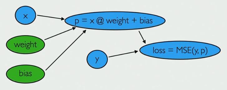
  • PyTorch helps us track computations through DAGs ML DAG
  • Loss (Mean Squared Error) depends on a lot of things, so loss is what we try to optimize
  • Stochastic gradient descent is doing gradient descent in shuffled batches so that we can minimize issues with not enough RAM
  • The df.pivot function can reformat tables!
  • To use PyTorch for ML, we want to have a DataSet (ds) and a DataLoader (dl)
    • The DataSet is a clean, raw representation of the data that we are using
    • The DataLoader basically helps enumerate and access the DataSet
      • Can help with creating batches and shuffling
basic training loop
model = torch.nn.Linear(1, 1)
optimizer = torch.optim.SGD([model.weight, model.bias], lr=0.00001)
loss_fn = torch.nn.MSELoss()
 
for epoch in range(50):
    for batchx, batchy in dl:
        predictedy = model(batchx)
        loss = loss_fn(batchy, predictedy)
        loss.backward()   # update weight.grad and bias.grad
        optimizer.step()  # update weight and bias based on gradients
        optimizer.zero_grad()  # weight.grad = 0 and bias.grad = 0
 
    # how well are we doing?
    x, y = ds[:]
    print(epoch, loss_fn(y, model(x)))

(threads)

  • Simple Python programs use at most ONE core so speed is capped by how much work one core can do
  • A process is a running program which has its own virtual address space (VAS)
    • The process cannot directly access physical memory
    • A VAS can have holes Processes and address spaces
  • A CPU core can be pointed at one instruction in the code at any time
    • Each core has its own cache
  • Threads have their own instruction pointers and stacks, but share the heap
    • Single-threaded processes have one pointer, multi-threaded processes have multiple pointers
  • Context switch: switching between threads — doing it too much is slow Context switch
  • Race conditions: when two threads both access a shared variable and problems occur

(locks)

  • Two threads can be interleaved and executed in a way that causes information to be lost
    • Modifying global variables and loading/storing simultaneously
  • We want atomicity — if it happens, then it happens together (otherwise not at all)
  • A lock (threading.Lock()) is held by only one thread at a time and protects critical sections from being inturrupted
    • Putting locks in the wrong places can still cause errors so the importantthing is to be careful / generous with where you’re putting locks
    • Locking and releasing is also an expensive operation!
  • If an exception occurs before the lock is released, then the code will never execute because the lock is still active
    • Use with statements

network resources

(RPC)

  • Every Network Interface Controller (NIC) has their own unique Media Access Control (MAC) address
    • Some devices randomly change or mask their MAC addresses for privacy (there are some good papers on this)
    • Computers can only send messages to other computers which are on the same network
  • An internet is just a group of networks; the Internet is the global one…?
  • A packet is a group of bytes that has an IP address which is its destination location
  • Private networks allow for duplicate IPv4 addresses private networks example
  • Network Address Translation (NAT) boxes can help you forward public IP addresses into private IP addresses in a network
  • Different port numbers on the same IP address can be running different servers
  • There are two main transport protocols:
    • TCP: reliable - will guarantee that the message is sent in the original order and will try to resend lost packets
    • UDP: unreliable - doesn’t do extra work, just sends the packet
  • HTTP methods: POST (create new), PUT (update), GET (fetch), DELETE for dealing with HTTP messages
  • RPC stands for Remote Procedure Call — calling a function remotely
    • gRPC, which helps with calling functions on a server, is built on top of HTTP
  • With RPCs, the code can be in different languages, so there needs to be a universal representation for types
    • Serialize (encode) and deserialize (decode) the types using a table — this is called protobufs
    • What do we have to take into consideration? Types, byte order, encoding length protobuf table
  • Make a .proto file to define messages that are being sent between two computers, then run gRPC on it to create classes
    • The classes are automatically generated in the specified language
    • The messages are basically objects that you can create
Example proto file for multiplying two numbers together
syntax = "proto3";
 
service Calc {
    rpc Mult(MultReq) returns (MultResp)
}
 
message MultReq {
    int32 x = 1;
    int32 y = 2;
}
 
message MultResp {
    int32 result = 1;
}
  • To call a function, you have to define an RPC in the format rpc NAME(ARGUMENTS), returns (RETURN VALUE); as a part of a service inside the .proto file

storage resources

(file systems)

  • Block devices are long term storage devices that are accessed in units of blocks
  • Caching is for storing data that might be accessed later, buffers mostly pertain to minimizing function calls for the same data, storing one large block/page of data when lines are being read one at a time
  • Small reads (<4KB):
    • No good way to read only one column without also reading everything else
    • The whole block has to be accessed to get a small portion of data
  • Hard disk drives (HDDs):
    • Steps to transfer data:
      1. Move pointer to correct track
      2. Wait for disk to rotate until data is under head
      3. Transfer data
    • For transferring small amounts of data, then the first two steps will dominate the processing time
    • Solution: assign sequential block numbers for HDDs
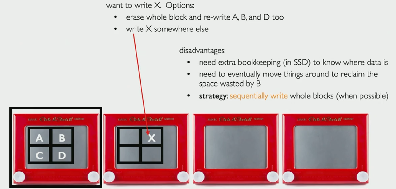
  • Solid state drives (SSDs):
    • No moving parts and can read data in parallel
    • Blocks and pages are used in different context than HDDs
    • Erase content in blocks, write content in pages, but can’t rewrite to individual pages
    • To rewrite content, SSDs just put it somewhere else and it needs to be tracked rewriting SSDs
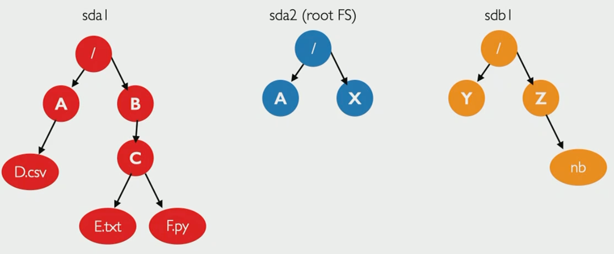
  • Block devices can be divided into partitions
  • Redundant Array of Inexpensive Disks (RAID) controllers can make multiple devices look like one device
  • Local file systems can track files by segmenting them into blocks and tracking which blocks are relevant to the file — this is called an inode structure
    • Directories contain inode mappings and names of files
  • Each drive has its own file system “tree” file tree

(formats and DBs)

  • Files store sequenes of bytes, but how do we organize the bytes in a useful format?
    • CSVs are row oriented
    • Parquets are column oriented
  • Choosing a file format depends on how we want to access the data
    • Transactions processing: reading or writing rows as needed
    • Analytics processing: computation over many rows to get specific columns
  • Parquets are much faster and the preferred data type for analytics processing!
  • Protobufs are the best way to get the smallest amount of bytes used for a piece of data
  • Compression is the idea of avoiding repetition in datasets
    • Parquets use snappy compression which prioritizes high speed over maximum compression
  • Schema is the structure of the dataset, like the types and field names
  • Databases have a bunch of tables which a user can query to get specific data back
    • SQL is the most popular querying language
    • Large DBs are usually only fast at either transactions or analytics, but not both
    • DB types: online transactions processing (OLTP) typically row oriented, online analytics processing (OLAP) typically column oriented
    • Extract-transform-load (ETL) is the process of transferring data from OLTPs into OLAPs dbms

clusters and hadoop ecosystem

further reading

  • Linear Algebra and Learning From Data by Gilbert Strang
  • Machine Learning with PyTorch and Scikit-Learn